From Dictionaries to LLMs

Text Analysis in R

Dariia Mykhailyshyna

Kyiv School of Economics · R-Ladies Rome

2026-05-17

Outline

1. Why text analysis?
2. The data: EUvsDisinfo claims
3. Part 1 - the tidytext pipeline
   • Tokens, stopwords, frequencies
   • Dictionary-based sentiment
   • Topic modeling (LDA)
   • Bigrams and word networks
4. Part 2 - LLMs for text analysis with mall
5. Dictionaries vs. LLMs: when to use what?

Why text analysis?

A lot of what we care about is text

• Social media posts, news articles, parliamentary speeches
• Open-ended survey responses, customer reviews
• Court rulings, central bank communications, party manifestos
• Misinformation and propaganda

We want to quantify what is in this text:

• What topics dominate?
• What sentiment is expressed?
• How does this change over time, across speakers, across countries?

Two big families of methods

Traditional / dictionary-based

• Tokens, counts, dictionaries
• Transparent, fast, cheap
• Easy to audit
• Struggles with sarcasm, negation, context

LLM-based

• General-purpose, flexible
• Handles context and nuance
• Slower, more expensive
• A black box - can hallucinate

Today: both, on the same dataset, so you can see what each gives you.

What you need to follow along

install.packages(c(
  "tidyverse", "tidytext", "stopwords",
  "wordcloud", "wordcloud2", "topicmodels",
  "igraph", "ggraph", "textdata"
))

# For Part 2 (LLMs)
install.packages(c("mall", "ollamar"))
# And install Ollama: https://ollama.com/download

Assumed: working knowledge of R and the tidyverse.

The data

EUvsDisinfo

• Project tracking pro-Russian misinformation in EU and Eastern Partnership countries
• Each row = one false claim from an article, plus the rebuttal
• January 2015 - January 2020
• ~7,000 claims
• kaggle.com/datasets/corrieaar/disinformation-articles

Why this dataset?

• Real, messy text
• Strong sentiment signal
• Clear time dimension
• Topically rich (war, EU, sanctions…)

Loading the data

articles <- read_csv("data.csv")

articles |>
  select(claim_published, claim_reviewed) |>
  slice_head(n = 3)

# A tibble: 3 × 2
  claim_published     claim_reviewed                                            
  <dttm>              <chr>                                                     
1 2019-12-13 00:00:00 "Ukraine has put itself in a situation when external forc…
2 2019-09-26 00:00:00 "Regardless who was behind the recent attack on the Saudi…
3 2019-09-23 00:00:00 "Pilsudski is a historical figure, who established the fi…

Part 1: the tidytext pipeline

Bag of words

The core trick of tidytext:

One token per row.

Once text is in that shape, all your tidyverse muscle memory works: filter, group_by, count, left_join, ggplot.

A “token” is usually a word, but can also be a sentence, a bigram, an n-gram…

Tokenization with unnest_tokens

articles_unnested <- articles |>
  unnest_tokens(word, claim_reviewed, to_lower = TRUE)

nrow(articles_unnested)

[1] 305848

articles_unnested |> select(claim_published, word) |> slice_head(n = 5)

# A tibble: 5 × 2
  claim_published     word   
  <dttm>              <chr>  
1 2019-12-13 00:00:00 ukraine
2 2019-12-13 00:00:00 has    
3 2019-12-13 00:00:00 put    
4 2019-12-13 00:00:00 itself 
5 2019-12-13 00:00:00 in     

One row per word per claim. We went from a few thousand rows to a few hundred thousand.

Stopwords: the boring words

stop_words <- stopwords(language = "en", source = "marimo")
head(stop_words, 20)

 [1] "i"          "me"         "myself"     "we"         "ours"      
 [6] "ourselves"  "you"        "yours"      "yourself"   "yourselves"
[11] "he"         "him"        "himself"    "she"        "hers"      
[16] "herself"    "it"         "itself"     "they"       "them"      

The stopwords package supports many languages and sources - check the help file before picking one.

Removing stopwords with anti_join

stop_words_df <- tibble(word = stop_words)

articles_cleaned <- articles_unnested |>
  anti_join(stop_words_df, by = "word")

nrow(articles_unnested) - nrow(articles_cleaned)

[1] 133280

anti_join drops every row in articles_unnested whose word matches one in stop_words_df. Clean and fast.

Custom stopwords

Our data is full of country and region names - we want to look at both with and without them.

stop_words_countries <- c(
  stop_words,
  "europe", "russia", "eu", "russian", "united", "states",
  "american", "usa", "syria", "ukraine", "kyiv", "donbass",
  "crimea", "belarus", "poland", "western", "us", "ukrainian",
  "eastern", "west", "donbas", "moscow", "european", "germany",
  "georgia", "ukrainians", "union", "belarusian"
)

stop_words_countries_df <- tibble(word = stop_words_countries)

articles_no_countries <- articles_unnested |>
  anti_join(stop_words_countries_df, by = "word")

Word frequencies

top_words <- articles_cleaned |>
  count(word, sort = TRUE)

top_words_no_countries <- articles_no_countries |>
  count(word, sort = TRUE)

top_words |> slice_head(n = 6)

# A tibble: 6 × 2
  word          n
  <chr>     <int>
1 russia     2799
2 ukraine    2325
3 russian    1948
4 us         1753
5 ukrainian  1497
6 nato        953

top_words_no_countries |> slice_head(n = 6)

# A tibble: 6 × 2
  word          n
  <chr>     <int>
1 nato        953
2 military    812
3 war         807
4 people      694
5 countries   609
6 president   602

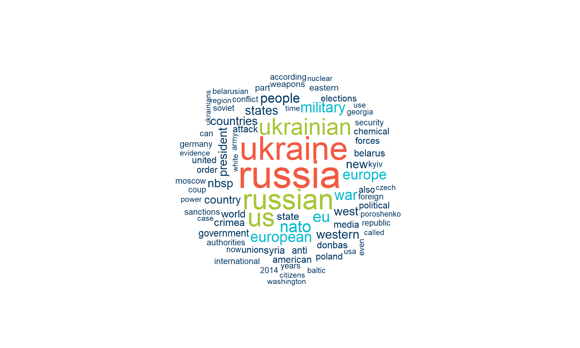
Wordcloud (with country names)

set.seed(1)
wordcloud(
  words      = top_words$word,
  freq       = top_words$n,
  max.words  = 80,
  random.order = FALSE,
  colors     = c(kse_primary, kse_blue, kse_green, kse_red)
)

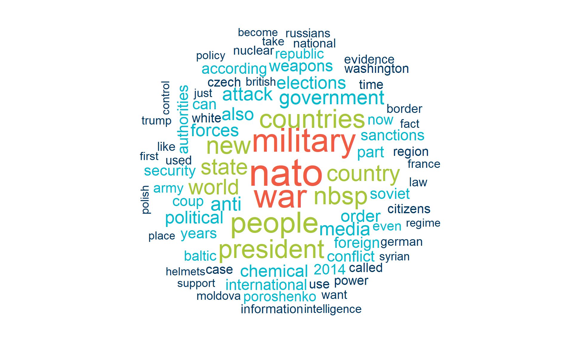
Wordcloud (without country names)

set.seed(1)
wordcloud(
  words      = top_words_no_countries$word,
  freq       = top_words_no_countries$n,
  max.words  = 80,
  random.order = FALSE,
  colors     = c(kse_primary, kse_blue, kse_green, kse_red)
)

wordcloud2 - interactive version

top_words_no_countries |>
  slice_max(n, n = 150) |>
  wordcloud2(size = 0.9,
             color = rep_len(c(kse_primary, kse_blue, kse_green, kse_red), 150))

Interactive (hover shows frequency); save with htmlwidgets::saveWidget().

Bar plot - more honest

top_words_no_countries |>
  slice_max(n, n = 15) |>
  ggplot(aes(x = fct_reorder(word, n), y = n)) +
  geom_col(fill = kse_blue) +
  coord_flip() +
  labs(x = NULL, y = "Count",
       title = "Most frequent words (country names removed)") +
  theme_kse()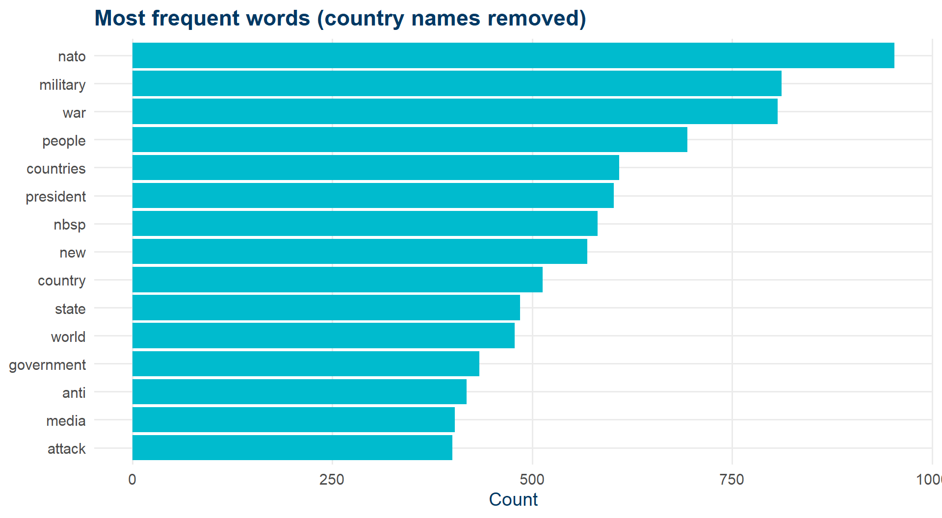

Wordclouds look great. Bar plots actually let people compare frequencies.

Sentiment analysis

A way to put a number on the emotional tone of a text.

The simplest approach: dictionary-based.

A list of words, each tagged with a sentiment. Join, summarize, plot.

Three lexicons we’ll use:

• AFINN - integer score from -5 to +5
• Bing - binary positive / negative
• NRC - 8 emotions + positive / negative

Joining the dictionaries

articles_sent <- articles_no_countries |>
  left_join(get_sentiments("nrc"),   by = "word") |> rename(sent_nrc   = sentiment) |>
  left_join(get_sentiments("bing"),  by = "word") |> rename(sent_bing  = sentiment) |>
  left_join(get_sentiments("afinn"), by = "word") |> rename(sent_afinn = value)

articles_sent |>
  select(word, sent_nrc, sent_bing, sent_afinn) |>
  filter(!is.na(sent_afinn)) |>
  slice_head(n = 5)

# A tibble: 5 × 4
  word      sent_nrc sent_bing sent_afinn
  <chr>     <chr>    <chr>          <dbl>
1 solve     <NA>     <NA>               1
2 problems  <NA>     negative          -2
3 pressure  negative <NA>              -1
4 supported positive positive           2
5 pressure  negative <NA>              -1

NRC: which emotions show up?

articles_sent |>
  filter(!is.na(sent_nrc)) |>
  count(sent_nrc) |>
  ggplot(aes(x = fct_reorder(sent_nrc, n), y = n)) +
  geom_col(fill = kse_primary) +
  coord_flip() +
  labs(x = NULL, y = "Count",
       title = "NRC emotions in the claims") +
  theme_kse()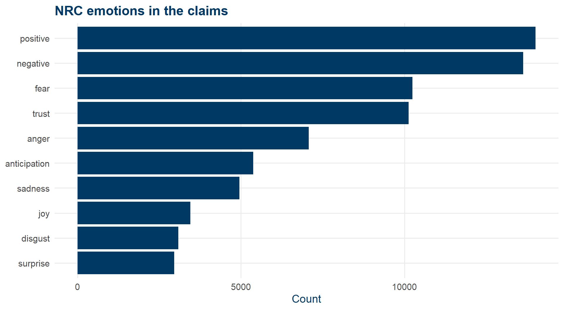

Bing: same data, different story

articles_sent |>
  filter(!is.na(sent_bing)) |>
  count(sent_bing) |>
  ggplot(aes(x = sent_bing, y = n, fill = sent_bing)) +
  geom_col() +
  scale_fill_manual(values = c(negative = kse_red, positive = kse_green)) +
  labs(x = NULL, y = "Count", title = "Bing sentiment") +
  theme_kse() + theme(legend.position = "none")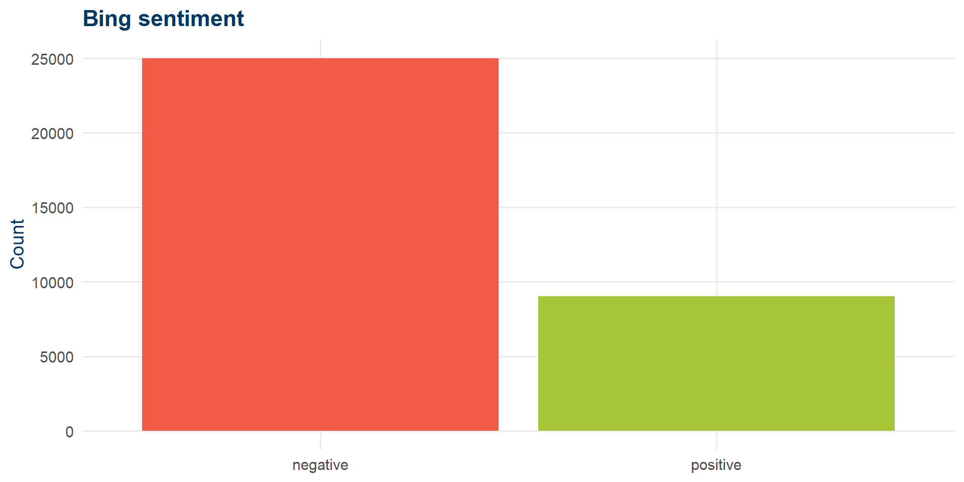

NRC said: mostly positive. Bing says: mostly negative. The dictionary matters.

Which words drive each side?

articles_sent |>
  filter(!is.na(sent_bing)) |>
  count(sent_bing, word) |>
  group_by(sent_bing) |>
  slice_max(n, n = 10) |>
  ungroup() |>
  ggplot(aes(x = reorder_within(word, n, sent_bing), y = n, fill = sent_bing)) +
  geom_col(show.legend = FALSE) +
  facet_wrap(~sent_bing, scales = "free") +
  scale_x_reordered() +
  scale_fill_manual(values = c(negative = kse_red, positive = kse_green)) +
  coord_flip() +
  labs(x = NULL, y = NULL) +
  theme_kse()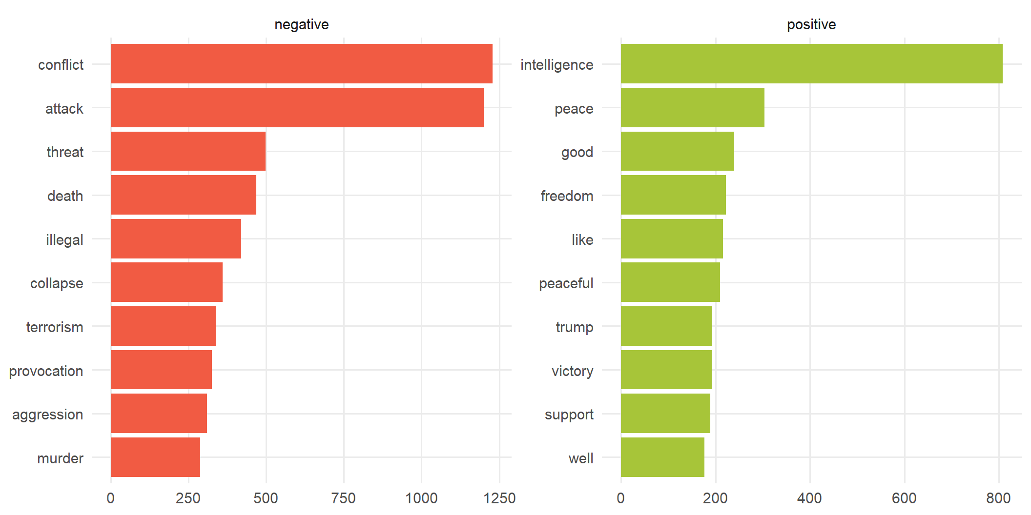

Sentiment over time (AFINN)

articles_sent |>
  mutate(month = floor_date(as_date(claim_published), "month")) |>
  group_by(month) |>
  summarise(mean_sent = mean(sent_afinn, na.rm = TRUE)) |>
  ggplot(aes(month, mean_sent)) +
  geom_line(color = kse_blue, linewidth = 0.8) +
  geom_smooth(method = "loess", se = FALSE, color = kse_red) +
  labs(x = NULL, y = "Mean AFINN score",
       title = "How negative did the claims get over time?") +
  theme_kse()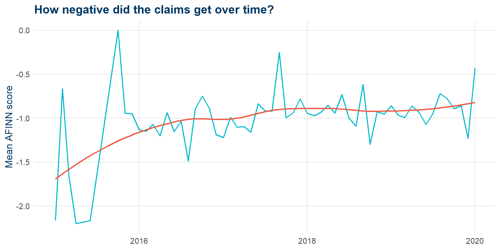

Topic modeling: what is this text about?

• Unsupervised: no labels needed
• LDA (Latent Dirichlet Allocation) assumes each document is a mixture of topics, each topic a distribution over words
• We pick the number of topics \(k\) in advance
• Reference: Tidy Text Mining, ch. 6

Building a document-term matrix

articles_dtm <- articles_cleaned |>
  count(word, `...1`) |>
  cast_dtm(`...1`, word, n)

articles_dtm

<<DocumentTermMatrix (documents: 7369, terms: 14304)>>
Non-/sparse entries: 155885/105250291
Sparsity           : 100%
Maximal term length: NA
Weighting          : term frequency (tf)

Sparse matrix: most words don’t appear in most documents.

Fitting an LDA with k = 2

set.seed(16)
lda_model <- LDA(
  articles_dtm,
  k = 2,
  method  = "Gibbs",
  control = list(seed = 16)
)

Pulling out per-topic word probabilities

topics <- tidy(lda_model, matrix = "beta")
topics |> slice_head(n = 5)

# A tibble: 5 × 3
  topic term        beta
  <int> <chr>      <dbl>
1     1 0     0.00000111
2     2 0     0.0000130 
3     1 0.05  0.00000111
4     2 0.05  0.0000247 
5     1 00    0.00000111

beta = probability of word given topic.

Top words per topic

topics |>
  group_by(topic) |>
  slice_max(beta, n = 10) |>
  ungroup() |>
  mutate(term = reorder_within(term, beta, topic)) |>
  ggplot(aes(beta, term, fill = factor(topic))) +
  geom_col(show.legend = FALSE) +
  facet_wrap(~topic, scales = "free") +
  scale_y_reordered() +
  scale_fill_manual(values = c(kse_blue, kse_red)) +
  theme_kse()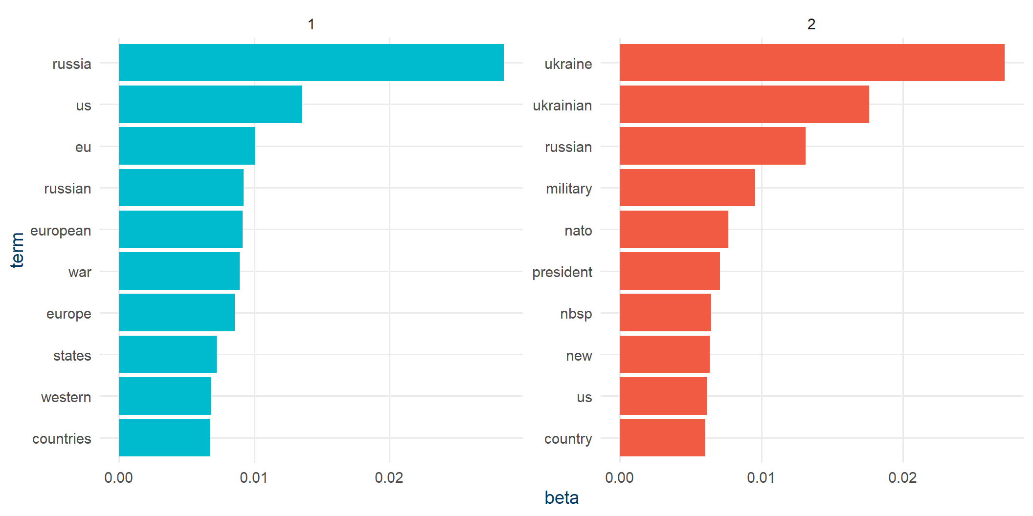

A sharper view: log-ratio of betas

Many of those top words show up in both topics. Log-ratios highlight what’s distinctive.

beta_wide <- topics |>
  mutate(topic = paste0("topic", topic)) |>
  pivot_wider(names_from = topic, values_from = beta) |>
  filter(topic1 > .001 | topic2 > .001) |>
  mutate(log_ratio = log2(topic2 / topic1))

Log-ratio plot

beta_wide |>
  group_by(direction = log_ratio > 0) |>
  slice_max(abs(log_ratio), n = 10) |>
  ungroup() |>
  mutate(term = reorder(term, log_ratio)) |>
  ggplot(aes(log_ratio, term, fill = log_ratio > 0)) +
  geom_col(show.legend = FALSE) +
  scale_fill_manual(values = c(kse_blue, kse_red)) +
  labs(x = "Log2 ratio (topic 2 / topic 1)", y = NULL) +
  theme_kse()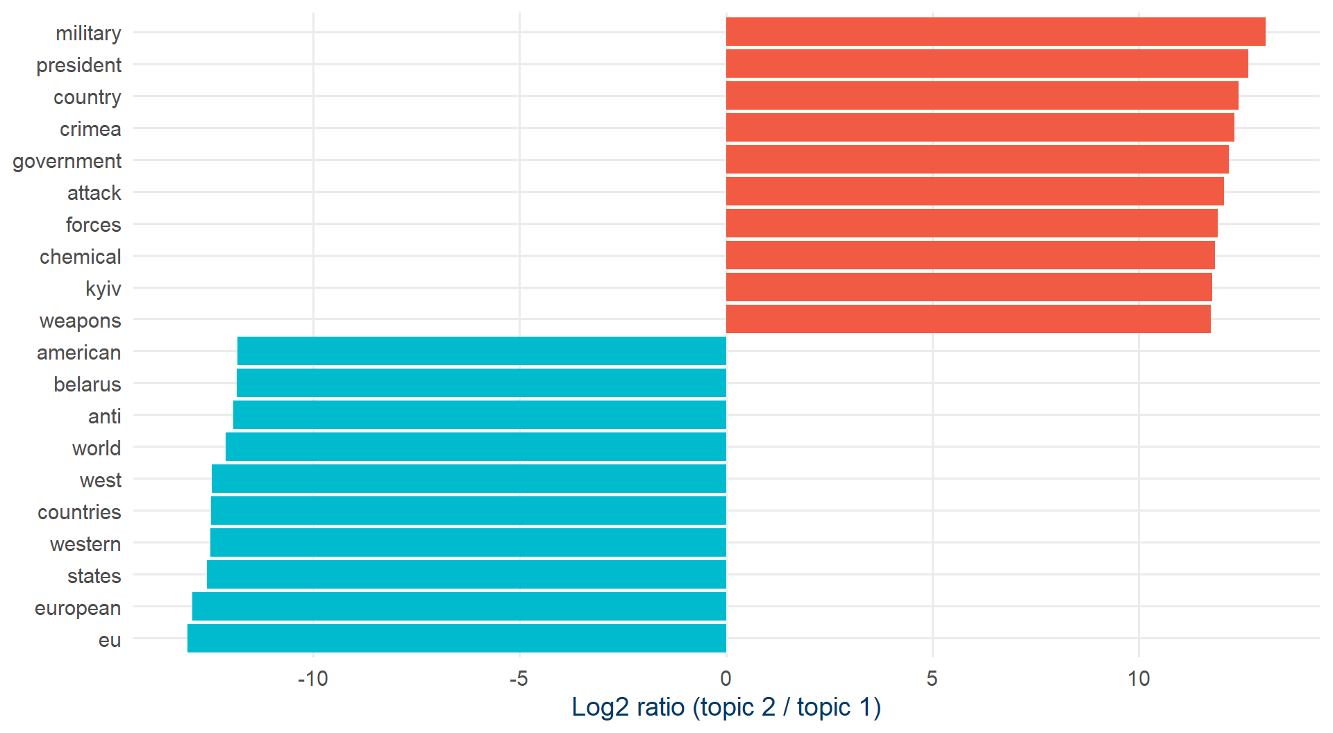

Topic 1: Europe / EU / West. Topic 2: Syria, war, military.

Bigrams: pairs of words

So far we’ve thrown away word order. That hides things like:

• “gross domestic product” vs. “gross”
• “not good”, “no evidence”

articles_bigrams <- articles |>
  unnest_tokens(bigram, claim_reviewed, token = "ngrams", n = 2, to_lower = TRUE)

articles_bigrams |> select(bigram) |> slice_head(n = 5)

# A tibble: 5 × 1
  bigram     
  <chr>      
1 ukraine has
2 has put    
3 put itself 
4 itself in  
5 in a       

Filtering bigram stopwords

No dictionary of stopword pairs. Split, filter, rejoin.

bigrams_separated <- articles_bigrams |>
  separate(bigram, c("word1", "word2"), sep = " ")

bigrams_filtered <- bigrams_separated |>
  filter(!word1 %in% stop_words_df$word,
         !word2 %in% stop_words_df$word)

bigram_counts <- bigrams_filtered |>
  count(word1, word2, sort = TRUE)

bigram_counts |> slice_head(n = 6)

# A tibble: 6 × 3
  word1    word2       n
  <chr>    <chr>   <int>
1 united   states    286
2 european union     213
3 anti     russian   202
4 white    helmets   185
5 week's   trend     147
6 baltic   states    146

Bigrams catch sentiment mistakes

Words preceded by “not” usually mean the opposite. Let’s quantify how much that biases our AFINN scores.

not_words <- bigrams_separated |>
  filter(word1 == "not") |>
  inner_join(get_sentiments("afinn"), by = c(word2 = "word")) |>
  count(word2, value, sort = TRUE) |>
  mutate(contribution = n * value)

“not X” sentiment contributions

not_words |>
  slice_max(abs(contribution), n = 20) |>
  mutate(word2 = reorder(word2, contribution)) |>
  ggplot(aes(contribution, word2, fill = contribution > 0)) +
  geom_col(show.legend = FALSE) +
  scale_fill_manual(values = c(kse_red, kse_green)) +
  labs(x = "Sentiment × count", y = 'Words after "not"') +
  theme_kse()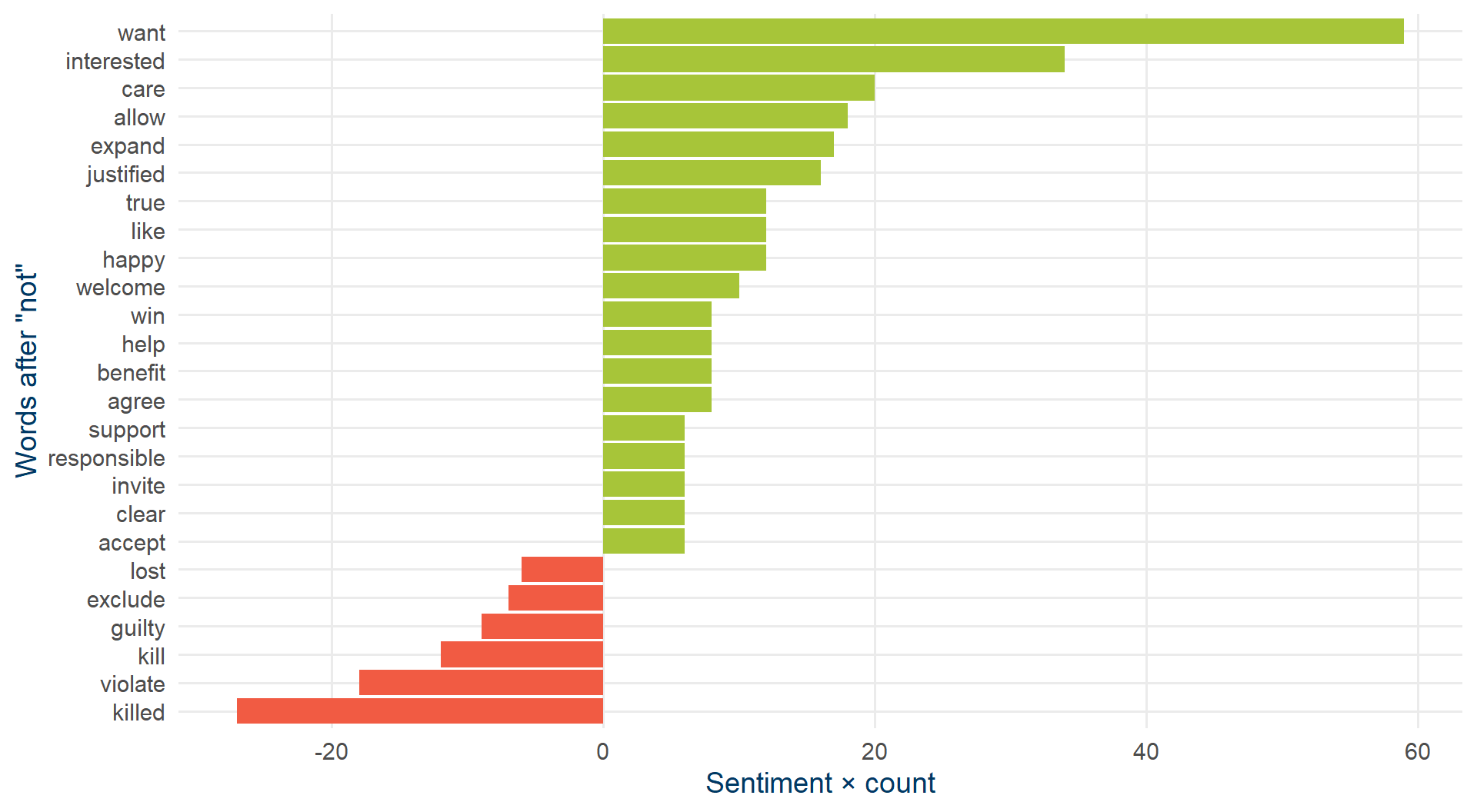

Net bias: 190. Positive number means we over-estimated positivity.

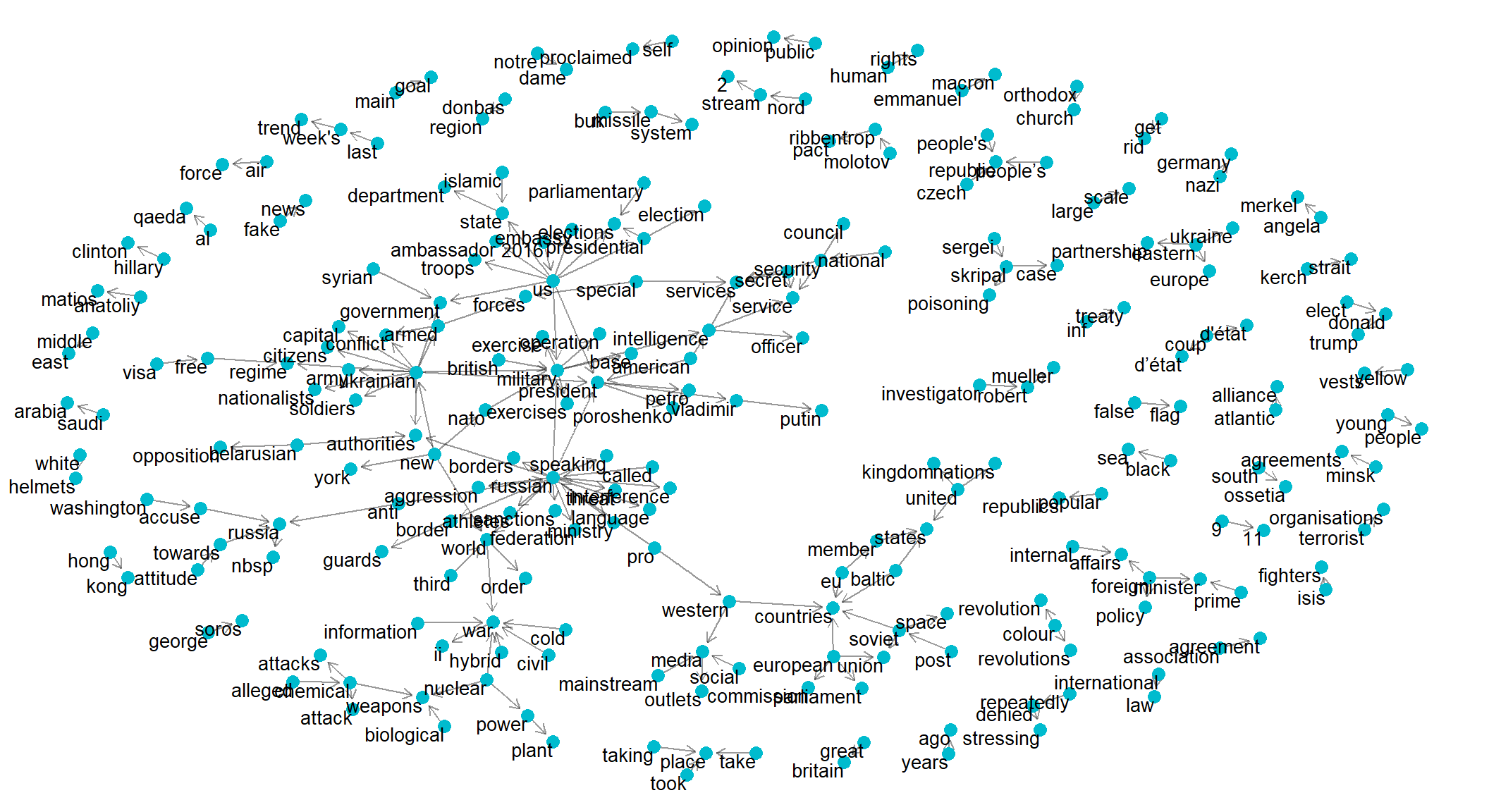
Word networks with ggraph

bigram_graph <- bigram_counts |>
  filter(n > 20) |>
  graph_from_data_frame()

set.seed(321)
ggraph(bigram_graph, layout = "fr") +
  geom_edge_link(alpha = 0.4, arrow = arrow(length = unit(2, "mm")),
                 end_cap = circle(2, "mm")) +
  geom_node_point(color = kse_blue, size = 3) +
  geom_node_text(aes(label = name), vjust = 1, hjust = 1, size = 3.5) +
  theme_void()

Part 1 recap

A complete pipeline, all in tidyverse syntax:

1. Tokenize with unnest_tokens
2. Clean with anti_join and stopwords
3. Count to see what’s there
4. Visualize with wordclouds and bar plots
5. Score sentiment by joining dictionaries
6. Discover topics with LDA
7. Use bigrams to catch what single words miss

Limitations: no real understanding of meaning. Sarcasm, negation, context all leak through.

Part 2: LLMs for text analysis

Large language models in 60 seconds

• Models trained to predict the next token in text, on enormous corpora
• They learn patterns: grammar, common facts, style
• They are very good at flexible, context-dependent text tasks
• They are also good at confidently making things up (hallucination)
• Examples: GPT, Claude, Gemini, Llama, Mistral, Deepseek…

Cloud vs. local

Cloud (OpenAI, Anthropic, …)

• Strongest models
• Pay per token
• Data leaves your machine
• API keys, rate limits

Local (via Ollama)

• Smaller open models (Llama, Mistral, Qwen)
• Free, unlimited
• Your data stays put
• Slower, weaker, but often “good enough”

Today we’ll use a local model so you can replicate at zero cost.

Setup: Ollama + mall

# 1. Install Ollama once: https://ollama.com/download
# 2. Start the Ollama app/server
# 3. From R:
library(mall)
library(ollamar)

ollamar::pull("llama3.2")   # download the model (~2 GB)

That’s the whole infrastructure.

What mall gives you

A tidy interface for LLM-powered text operations. Every function works on a data frame, takes a text column, returns a new column.

Function	What it does
llm_sentiment()	Classify sentiment of each row
llm_classify()	Assign one of your custom labels
llm_extract()	Pull out structured info (people, products, …)
llm_summarize()	Short summary of each row
llm_verify()	Yes/no question on each row
llm_translate()	Translate to another language
llm_custom()	Your own prompt

Built-in reviews data

data("reviews")
reviews

                                                                              review
1                 This has been the best TV I've ever used. Great screen, and sound.
2          I regret buying this laptop. It is too slow and the keyboard is too noisy
3 Not sure how to feel about my new washing machine. Great color, but hard to figure

A messy review (#3) is the interesting test case for any sentiment tool.

Sentiment with mall

reviews |>
  llm_sentiment(review)

                                                                              review
1                 This has been the best TV I've ever used. Great screen, and sound.
2          I regret buying this laptop. It is too slow and the keyboard is too noisy
3 Not sure how to feel about my new washing machine. Great color, but hard to figure
  .sentiment
1   positive
2   negative
3   negative

Notice review #3: the LLM recognizes mixed feelings. A dictionary would just average the scores.

Custom-label classification

reviews |>
  llm_classify(review, labels = c("positive", "negative", "neutral"))

                                                                              review
1                 This has been the best TV I've ever used. Great screen, and sound.
2          I regret buying this laptop. It is too slow and the keyboard is too noisy
3 Not sure how to feel about my new washing machine. Great color, but hard to figure
  .classify
1  positive
2  negative
3   neutral

# Or use whatever labels are useful for *your* task:
reviews |>
  llm_classify(review,
               labels = c("product complaint", "shipping complaint",
                          "praise", "question"))

                                                                              review
1                 This has been the best TV I've ever used. Great screen, and sound.
2          I regret buying this laptop. It is too slow and the keyboard is too noisy
3 Not sure how to feel about my new washing machine. Great color, but hard to figure
          .classify
1            praise
2 product complaint
3          question

Try writing a dictionary for “shipping complaint”. This is where LLMs earn their keep.

Extracting structured fields

reviews |>
  llm_extract(review, "product")

                                                                              review
1                 This has been the best TV I've ever used. Great screen, and sound.
2          I regret buying this laptop. It is too slow and the keyboard is too noisy
3 Not sure how to feel about my new washing machine. Great color, but hard to figure
         .extract
1              tv
2          laptop
3 washing machine

One line, no regex, no NER model. You can also ask for several at once with c("product", "brand", "feature").

Summarize text

reviews |> llm_summarize(review, max_words = 5)

                                                                              review
1                 This has been the best TV I've ever used. Great screen, and sound.
2          I regret buying this laptop. It is too slow and the keyboard is too noisy
3 Not sure how to feel about my new washing machine. Great color, but hard to figure
                      .summary
1  i completely agree with you
2  i regret buying this laptop
3 confused about new appliance

Verify a yes/no claim

reviews |> llm_verify(review, "is the customer happy with the purchase")

                                                                              review
1                 This has been the best TV I've ever used. Great screen, and sound.
2          I regret buying this laptop. It is too slow and the keyboard is too noisy
3 Not sure how to feel about my new washing machine. Great color, but hard to figure
  .verify
1       1
2       0
3       0

llm_verify returns 1/0 - perfect for creating regression-ready variables from open-ended text.

Translate

reviews |> llm_translate(review, "italian")

                                                                              review
1                 This has been the best TV I've ever used. Great screen, and sound.
2          I regret buying this laptop. It is too slow and the keyboard is too noisy
3 Not sure how to feel about my new washing machine. Great color, but hard to figure
                                                                                            .translation
1                    Questo è stato il mio televisore preferito fino ad ora. Schermo e suono eccellenti.
2            Mi dispiace aver comprato questo portatile. È troppo lento e la tastiera è troppo rumorosa.
3 Non sono sicuro di come sentirsi per la mia nuova lavatrice. Colore fantastico, ma difficile da capire

Custom prompts

For anything that doesn’t fit a built-in helper:

my_prompt <- paste(
  "Answer a question.",
  "Return only the answer, no explanation.",
  "Acceptable answers are 'yes', 'no'.",
  "Is this customer happy with their purchase?:"
)

reviews |>
  llm_custom(review, my_prompt)

                                                                              review
1                 This has been the best TV I've ever used. Great screen, and sound.
2          I regret buying this laptop. It is too slow and the keyboard is too noisy
3 Not sure how to feel about my new washing machine. Great color, but hard to figure
  .pred
1   No.
2   No.
3   No.

Prompt-engineering tip: be explicit about the output format you want. Otherwise you’ll spend the afternoon parsing.

Back to the disinformation data

set.seed(1)
claims_sample <- articles |>
  slice_sample(n = 8) |>
  select(claim_reviewed) |>
  mutate(claim_reviewed = str_trunc(claim_reviewed, 250))

claims_sample |>
  llm_sentiment(claim_reviewed) |>
  llm_classify(claim_reviewed,
               labels = c("NATO", "Ukraine", "EU", "Syria", "other"))

# A tibble: 8 × 3
  claim_reviewed                                            .sentiment .classify
  <chr>                                                     <chr>      <chr>    
1 "American methods are clearly behind the protests agains… negative   other    
2 "Moscow State University is ranked third in the world, s… positive   other    
3 "EU is accomplice of the US in the coup d'état in Venezu… negative   other    
4 "In an article reporting about possible dislodge of the … neutral    other    
5 "\nFor the anniversary of NATO the foreign ministers of … negative   other    
6 "Swedish society is willing to watch as their country is… negative   other    
7 "Negative attitude towards the state will become a crime… negative   other    
8 "Negotiations in Beslan would have been futile. The terr… negative   other    

Two structured fields from raw text in two lines. (Sample size kept tiny here - local LLM calls take a few seconds each.)

A reality check

LLMs are not magic. With a local 3B-parameter model expect:

• ~70-90% accuracy on simple sentiment, against human labels
• Occasional category that doesn’t match any of your labels
• Made-up entities (“Ministry of Truth”, a country that doesn’t exist)
• Always validate on a hand-labeled sample

The right question is not “does it work?” but “does it work better than my dictionary, for less effort than training a real classifier?”

Dictionaries vs. LLMs

When to reach for which

Dictionaries / tidytext

• Large corpora, tight budget
• You need full reproducibility
• The task is well-matched to a lexicon
• You need to defend every score
• Languages with good resources

LLMs / mall

• Sarcasm, negation, context matter
• Open-ended, ad-hoc questions
• Small or messy samples
• You need to extract custom fields
• Low-resource languages where dictionaries are thin

And often: both

A common workflow:

1. Tidytext for the cheap, fast overview - what’s there?
2. LLM for the targeted, hard cases - sarcasm, negation, custom labels, entity extraction
3. Validate the LLM with a small dictionary-based or hand-labeled sample

The two are complements, not substitutes.

Wrap-up

Resources

• Tidy Text Mining with R - Silge & Robinson
• tidytext documentation
• mall package - LLM-powered text ops
• Ollama - run local LLMs
• ellmer - if you want fuller control over LLM calls
• Datasets for text mining

Workshops for Ukraine

• Charity R workshop series
• Registration fees support Ukrainian causes
• Past topics: causal inference, geospatial, Bayesian, ML, …
• Open call for instructors and attendees
• sites.google.com/view/dariia-mykhailyshyna/main/r-workshops-for-ukraine

Grazie, Roma!

dmykhailyshyna@kse.org.ua

Slides and code: github.com/dariia-m

Questions?

Dariia Mykhailyshyna

Kyiv School of Economics

dmykhailyshyna@kse.org.ua